Introducing the ecoengine package

Natural history museums have long been valuable repositories of data on species diversity. These data have been critical for fostering and shaping the development of fields such as biogeography and systematics. The importance of these data repositories is becoming increasingly important, especially in the context of climate change, where a strong understanding of how species responded to past climate is key to understanding their responses in the future. Leading the way in opening up such valuable data is a new effort by the Berkeley Initiative in Global Change Biology called the Ecoengine.

The engine is a fast and open API that provides access to over 3 million specimens and vegetation data from surveys. Many of these specimens have already been georeferenced opening up several use cases for such data. In addition, the engine also provides access to species checklists and sensor data from the Keck Hydrowatch project from the Eel river field station. Our newest package, ecoengine, provides an easy interface to these data.

🔗 Installing the package

A stable version of the package (1.1) is now available on CRAN. To install:

install.packages("ecoengine")
# A small bug with factors (to be resolved in a couple of days in 1.1.2) requires strings as factors to be FALSE
options(stringsAsFactors = FALSE)

You can also install a development version of the package that has additional features (more below), with several new updates that will appear on the next CRAN version (ETA mid-March). To install the development version:

library(devtools)
install_github("ropensci/ecoengine")

Observation data

The workhorse function of the package is ee_observations() which provides a way to query any taxonomic field. Searches for any field are automatically fuzzy but one can request exact searches by adding __exact (note the two underscores) to any field being searched. So for example, if you are interested in data on the genus lynx, one can query those data like so:

library(ecoengine)
lynx_data <- ee_observations(genus = "lynx", progress = FALSE)

## Search contains 795 observations (downloading 1 of 1 pages)

lynx_data

## [Total results]: 795
## [Args]:
## country = United States
## genus = lynx
## georeferenced = FALSE
## page_size = 25
## page = 1
## [Type]: observations
## [Number of results]: 25

All ecoengine queries are returned as S3 objects of class ecoengine. The object includes a total number of results available, the arguments used (so someone else can reconstruct the same query), the type of data returned (photos, observations, checklists, sensor), and the actual data itself. The results are paginated to prevent large requests from hanging part way. Each call returns 25 observations (can be overridden) and one can request more data by passing a page argument (e.g. page = 1). Pages can also be ranges, or “all” to request all available data for a query. The pagination method allows calls to be parallelized and reassembled easily, especially when requests may return tens of thousand of records. In this case there are only 795 records so we can request everything in one go.

library(ecoengine)
lynx_data <- ee_observations(genus = "lynx", progress = FALSE, page = "all")

## Search contains 795 observations (downloading 32 of 32 pages)

# The progress bar is useful on the command line but tends to clutter up
# documentation which is why it’s been turned off here. Messages can also be
# turned off with quiet = TRUE
lynx_data

## [Total results]: 795
## [Args]:
## country = United States
## genus = lynx
## georeferenced = FALSE
## page_size = 25
## page = all
## [Type]: observations
## [Number of results]: 795

Other fields (all documented and available from ?ee_observations) include kingdom, phylum, clss (intentionally misspelled to avoid conflict with a sql keyword), genus and scientific_name. Any of these fields can also be searched exactly by adding __exact at the end.

We can request georeferenced data only for visualization purposes.

lynx_data <- ee_observations(genus = "lynx", progress = FALSE, page = "all",
    georeferenced = TRUE)

## Search contains 714 observations (downloading 29 of 29 pages)

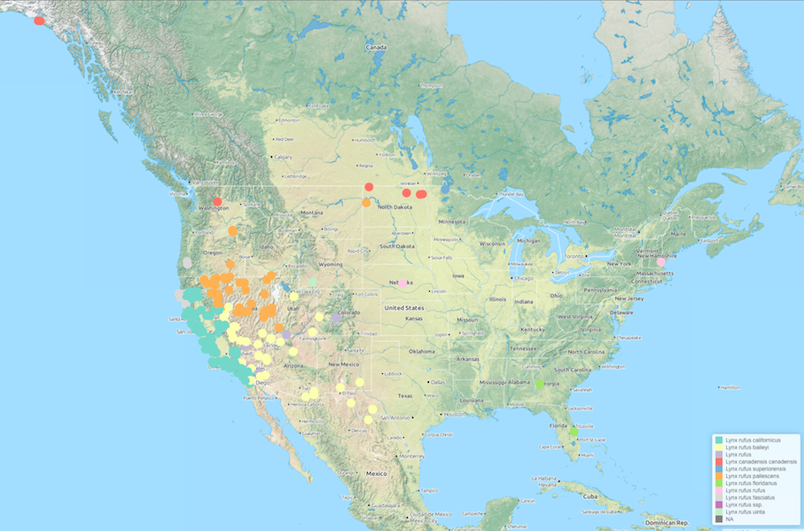
and it’s easy to examine these data as an interactive map using the ee_map function (the function is currently only available in the dev version).

ee_map(lynx_data)

This generates an interactive Leaflet JS map and renders to your default browser. You can easily embed such maps into talks using iFrames and Slidify.

The search possibilities are endless and the data can be supplemented by many other sources in our site (e.g. taxize). Here are a few example queries.

pinus <- ee_observations(scientific_name = "Pinus")
lynx_data <- ee_observations(genus = "Lynx")
# Georeferenced data only
lynx_data <- ee_observations(genus = "Lynx", georeferenced = TRUE)
animalia <- ee_observations(kingdom = "Animalia")
Artemisia <- ee_observations(scientific_name = "Artemisia douglasiana")
asteraceae <- ee_observationss(family = "asteraceae")
vulpes <- ee_observations(genus = "vulpes")
Anas <- ee_observations(scientific_name = "Anas cyanoptera", page = "all")
loons <- ee_observations(scientific_name = "Gavia immer", page = "all")
plantae <- ee_observations(kingdom = "plantae")
chordata <- ee_observations(phylum = "chordata")
# Class is clss since the former is a reserved keyword in SQL.
aves <- ee_observations(clss = "aves")

Checklist data

The museum contains checklists of species spanning a long time scale. To query checklists, use ee_checklists()

all_lists <- ee_checklists()

## Returning 57 checklists

head(all_lists[, c("footprint", "subject")])

##                                                        footprint
## 1   https://ecoengine.berkeley.edu/api/footprints/angelo-reserve/
## 2   https://ecoengine.berkeley.edu/api/footprints/angelo-reserve/
## 3   https://ecoengine.berkeley.edu/api/footprints/angelo-reserve/
## 4 https://ecoengine.berkeley.edu/api/footprints/hastings-reserve/
## 5   https://ecoengine.berkeley.edu/api/footprints/angelo-reserve/
## 6 https://ecoengine.berkeley.edu/api/footprints/hastings-reserve/
##      subject
## 1    Mammals
## 2     Mosses
## 3    Beetles
## 4    Spiders
## 5 Amphibians
## 6       Ants

Currently there are 57 lists available. We can drill deeper into any list to get all the available data. We can also narrow our checklist search to groups of interest (see unique(all_lists$subject)). For example, to get the list of Spiders:

spiders <- ee_checklists(subject = "Spiders")

## Returning 2 checklists

spiders

##                  record
## 4  bigcb:specieslist:15
## 10 bigcb:specieslist:20
##                                                         footprint
## 4  https://ecoengine.berkeley.edu/api/footprints/hastings-reserve/
## 10   https://ecoengine.berkeley.edu/api/footprints/angelo-reserve/
##                                                                       url
## 4  https://ecoengine.berkeley.edu/api/checklists/bigcb%3Aspecieslist%3A15/
## 10 https://ecoengine.berkeley.edu/api/checklists/bigcb%3Aspecieslist%3A20/
##                                           source subject
## 4  https://ecoengine.berkeley.edu/api/sources/18/ Spiders
## 10 https://ecoengine.berkeley.edu/api/sources/18/ Spiders

Now we can drill deep into each list. For this tutorial I’ll just retrieve data from the the two lists returned above.

library(plyr)
spider_details <- ldply(spiders$url, checklist_details)
names(spider_details)

##  [1] "url"                              "observation_type"
##  [3] "scientific_name"                  "collection_code"
##  [5] "institution_code"                 "country"
##  [7] "state_province"                   "county"
##  [9] "locality"                         "coordinate_uncertainty_in_meters"
## [11] "begin_date"                       "end_date"
## [13] "kingdom"                          "phylum"
## [15] "clss"                             "order"
## [17] "family"                           "genus"
## [19] "specific_epithet"                 "infraspecific_epithet"
## [21] "source"                           "remote_resource"
## [23] "earliest_period_or_lowest_system" "latest_period_or_highest_system"

unique(spider_details$scientific_name)

##  [1] "holocnemus pluchei"        "oecobius navus"
##  [3] "uloborus diversus"         "neriene litigiosa"
##  [5] "theridion sp. A"           "tidarren sp."
##  [7] "dictyna sp. A"             "dictyna sp. B"
##  [9] "mallos sp."                "yorima sp."
## [11] "hahnia sanjuanensis"       "cybaeus sp."
## [13] "zanomys sp."               "anachemmis sp."
## [15] "titiotus sp."              "oxyopes scalaris"
## [17] "zora hespera"              "drassinella sp."
## [19] "phrurotimpus mateonus"     "scotinella sp."
## [21] "castianeira luctifera"     "meriola californica"
## [23] "drassyllus insularis"      "herpyllus propinquus"
## [25] "micaria utahna"            "trachyzelotes lyonneti"
## [27] "ebo evansae"               "habronattus oregonensis"
## [29] "metaphidippus sp."         "platycryptus californicus"
## [31] "calymmaria sp."            "frontinella communis"
## [33] "undetermined sp."          "latrodectus hesperus"
## [35] "theridion sp. B"           "agelenopsis oregonensis"
## [37] "pardosa spp."              "schizocosa mccooki"
## [39] "hololena sp."              "callobius sp."
## [41] "pimus sp."                 "aliatypus sp."
## [43] "antrodiaetus sp."          "antrodiaetus riversi"
## [45] "anyphaena californica"     "aculepeira packardi"
## [47] "araneus bispinosus"        "araniella displicata"
## [49] "cyclosa conica"            "cyclosa turbinata"
## [51] "brommella sp."             "cicurina sp."
## [53] "dictyna sp."               "emblyna oregona"
## [55] "orodrassus sp."            "sergiolus sp."
## [57] "erigone sp."               "pityohyphantes sp."
## [59] "tachygyna sp."             "alopecosa kochi"
## [61] "oxyopes salticus"          "philodromus sp."
## [63] "tibellus oblongus"         "pimoa sp."
## [65] "undetermined spp."         "metaphidippus manni"
## [67] "thiodina sp."              "diaea livens"
## [69] "metellina sp."             "cobanus cambridgei"
## [71] "tetragnatha sp."           "tetragnatha versicolor"
## [73] "dipoena sp."               "theridion spp."
## [75] "misumena vatia"            "misumenops sp."
## [77] "tmarus angulatus"          "xysticus sp."
## [79] "hyptiotes gertschi"        "mexigonus morosus"

Photo data

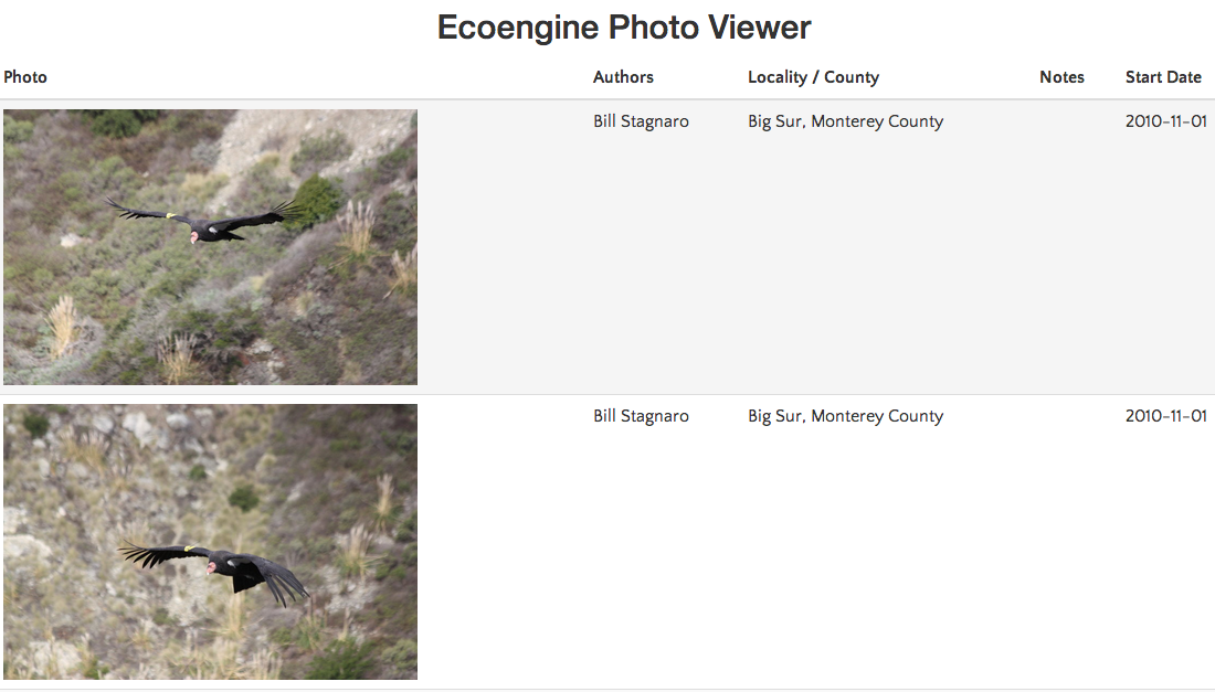
The ecoengine also contains a large number of photos from various sources. It’s easy to query the photo database using similar arguments as above. One can search by taxa, location, source, collection and much more. To get all pictures of the California condor from the database:

condor <- ee_photos(scientific_name = "Gymnogyps californianus", quiet = TRUE, progress = FALSE)

condor

## [Total results]: 8
## [Args]:
## page_size = 25
## scientific_name = Gymnogyps californianus
## georeferenced = FALSE
## page = 1
## [Type]: photos
## [Number of results]: 8

The package also provides functionality to quickly browse photos in the default browser. By calling view_photos() on any ecoengine object of type photos, R will render a static html page with thumbnails and metadata and launch a default browser with additional links.

view_photos(ee_photos(scientific_name = "Gymnogyps californianus", quiet = TRUE))

Sensor data

Sensor data come from the Keck HydroWatch Center. Retrieving the data are simple. Three functions provides all the necessary functionality.

• ee_list_sensors() - provides a list of sensors and the data they provide.
• ee_sensor_data() - retrieves data for any of these sensors (ids obtained by the previous function) and a date window.
• ee_sensor_agg - provides aggregated data that can be requested in any interval (minutes, days, weeks, months, years).

🔗 Searching the engine

The search is elastic by default. One can search for any field in ee_observations() across all available resources. For example,

# The search function runs an automatic elastic search across all resources
# available through the engine.
lynx_results <- ee_search(query = "genus:Lynx")
lynx_results[, -3]
# This gives you a breakdown of what's available allowing you dig deeper.

Upcoming features

In the next CRAN update we will add methods to retrieve all the vegetation data, the interactive maps, searching the data directly from the map (for example by drawing bounding boxes) and having a formatted query returned back to your R prompt for inclusion in a script.

As with all of our packages we welcome contributions to the GitHub repository as issues or pull requests.