September 11, 2018 From rOpenSci (https://deploy-preview-488--ropensci.netlify.app/blog/2018/09/11/birds-science/). Except where otherwise noted, content on this site is licensed under the CC-BY license.
In the second post of the series where we obtained data from eBird we determined what birds were observed in the county of Constance, and we complemented this knowledge with some taxonomic and trait information in the fourth post of the series. Now, we could be curious about the occurrence of these birds in scientific work. In this post, we will query the scientific literature and an open scientific data repository for species names: what have these birds been studied for? Read on if you want to learn how to use R packages allowing to do so!
🔗 Getting a list of 50 species from occurrence data
For more details about the following code, refer to the previous post of the series. The single difference is our adding a step to keep only data for the most recent years.
# polygon for filtering
landkreis_konstanz <- osmdata::getbb("Landkreis Konstanz",
                             format_out = "sf_polygon")
crs <- sf::st_crs(landkreis_konstanz)

# get and filter data
f_out_ebd <- "ebird/ebd_lk_konstanz.txt"

library("magrittr")

ebd <- auk::read_ebd(f_out_ebd) %>%
  sf::st_as_sf(coords = c("longitude", "latitude"),
                crs = crs)

in_indices <- sf::st_within(ebd, landkreis_konstanz)

ebd <- dplyr::filter(ebd, lengths(in_indices) > 0)

ebd <- as.data.frame(ebd)

ebd <- dplyr::filter(ebd, approved, lubridate::year(observation_date) > 2010)
For the sake of simplicity, we shall only use the 50 species observed the most often.
species <- ebd %>%
  dplyr::count(common_name, sort = TRUE) %>%
  head(n = 50) %>%
  dplyr::pull(common_name)
The species are Carrion Crow, Eurasian Blackbird, Mallard, Eurasian
Coot, Great Tit, Great Crested Grebe, Mute Swan, Great Cormorant,
Eurasian Blue Tit, Gray Heron, Black-headed Gull, Common Chaffinch,
Common Chiffchaff, Tufted Duck, European Starling, White Wagtail,
European Robin, Little Grebe, Common Wood-Pigeon, Red-crested Pochard,
Ruddy Shelduck, Graylag Goose, Red Kite, Common Buzzard, Eurasian
Blackcap, Great Spotted Woodpecker, Eurasian Magpie, Gadwall, Common
Pochard, Eurasian Nuthatch, Green-winged Teal, House Sparrow, Eurasian
Jay, Yellow-legged Gull, Yellowhammer, Eurasian Green Woodpecker, Eared
Grebe, Eurasian Reed Warbler, Barn Swallow, Northern Shoveler, Eurasian
Moorhen, Black Redstart, Great Egret, White Stork, Eurasian Wren,
Long-tailed Tit, Common House-Martin, Eurasian Kestrel, European
Goldfinch and European Greenfinch
(glue::glue_collapse(species, sep = ", ", last = " and ")).
🔗 Querying the scientific literature
Just like rOpenSci has a taxonomic toolbelt
(taxize) and a species
occurrence data toolbelt (spocc),
it has a super package for querying the scientific literature:
fulltext! This package
supports search for “PLOS via the rplos package, Crossref via the
rcrossref package, Entrez via the rentrez package, arXiv via the aRxiv
package, and BMC, Biorxiv, EuroPMC, and Scopus via internal helper
functions”.
We shall use fulltext to retrieve the titles and abstracts of
scientific articles mentioning each species, and will use tidytext to
compute the most prevalent words in these works.
We first define a function retrieving the titles and abstracts of works obtained as result when querying one species name.
We use dplyr::bind_rows because we want all results for one species at
once, while fulltext returns a list of data.frames with one data.frame
by data source.
.get_papers <- function(species){
  species %>%
    tolower() %>%
    fulltext::ft_search() %>%
    fulltext::ft_get() %>%
    fulltext::ft_collect() %>%
    fulltext::ft_chunks(c("title", "abstract")) %>%
    fulltext::ft_tabularize() %>%
    dplyr::bind_rows()
}

.get_papers(species[1]) %>%
  dplyr::pull(title)
##  [1] "Great spotted cuckoo nestlings have no antipredatory effect on magpie or carrion crow host nests in southern Spain"
##  [2] "Donor-Control of Scavenging Food Webs at the Land-Ocean Interface"
##  [3] "Formal comment to Soler et al.: Great spotted cuckoo nestlings have no antipredatory effect on magpie or carrion crow host nests in southern Spain"
##  [4] "Socially Driven Consistent Behavioural Differences during Development in Common Ravens and Carrion Crows"
##  [5] "Behavioral Responses to Inequity in Reward Distribution and Working Effort in Crows and Ravens"
##  [6] "Early Duplication of a Single MHC IIB Locus Prior to the Passerine Radiations"
##  [7] "Investigating the impact of media on demand for wildlife: A case study of Harry Potter and the UK trade in owls"
##  [8] "New Caledonian Crows Rapidly Solve a Collaborative Problem without Cooperative Cognition"
##  [9] "Nest Predation Deviates from Nest Predator Abundance in an Ecologically Trapped Bird"
## [10] "Dietary Compositions and Their Seasonal Shifts in Japanese Resident Birds, Estimated from the Analysis of Volunteer Monitoring Data"
If we were working on a scientific study, we’d add a few more filters,
e.g. having the species mentioned in the abstract, and not only
somewhere in the paper which is probably the way the different
literature search providers define a match. But we’re not, so we can
keep our query quite free! My favourite paper involving the Carrion Crow
is “Investigating the impact of media on demand for wildlife: A case
study of Harry Potter and the UK trade in
owls”
because it’s a fun and important scientific question, and is supported
by open data (by the way you can access CITES trade data (international
trade in endangered species) in R using
cites and CITES
Speciesplus database using
rcites).
We then apply this function to all 50 species and keep each article only once.
get_papers <- ratelimitr::limit_rate(.get_papers,
                                     rate = ratelimitr::rate(1, 2))

all_papers <- purrr::map_df(species, get_papers)

nrow(all_papers)
## [1] 522
all_papers <- unique(all_papers)

nrow(all_papers)
## [1] 378
Now, we get the most common words from titles and abstracts. For that we first append the title to the abstract which is a quick hack.
library("tidytext")
library("rcorpora")

stopwords <- corpora("words/stopwords/en")$stopWords

all_papers %>%
  dplyr::group_by(title, abstract) %>%
  dplyr::summarise(text = paste(title, abstract)) %>%
  dplyr::ungroup() %>%
  unnest_tokens(word, text) %>%
  dplyr::filter(!word %in% stopwords) %>%
  dplyr::count(word, sort = TRUE) -> words
So, what are the most common words in these papers?
head(words, n = 10)
##           word   n
## 1      species 754
## 2        birds 514
## 3        virus 270
## 4        avian 268
## 5         bird 262
## 6        study 243
## 7     breeding 231
## 8         wild 227
## 9  populations 217
## 10  population 213
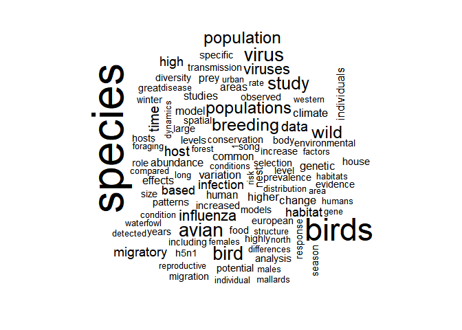
Not too surprising, and obviously less entertaining than looking at
individual species’ results. Maybe a wordcloud can give us a better idea
of the wide area of topics of studies involving our 50 most frequent
bird species. We use the wordcloud
package.
library("wordcloud")

with(words, wordcloud(word, n, max.words = 100))

We see that topics include ecological words such as “foraging” but also
epidemiological questions since “influenza” and “h5n1” come up. Now, how
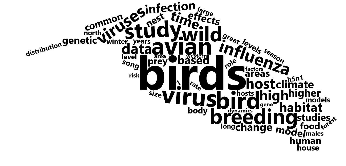
informative as this wordcloud can be, it’s a bit ugly, so we’ll prettify
it using the wordcloud2
package instead, and the
silhouette of a bird from
Phylopic.
bird <- words %>%
  head(n = 100) %>%
  wordcloud2::wordcloud2(figPath = "bird.png",
                       color = "black", size = 1.5)
# https://www.r-graph-gallery.com/196-the-wordcloud2-library/
htmlwidgets::saveWidget(bird,
                        "tmp.html",
                        selfcontained = F)
I wasn’t able to webshot the resulting html despite increasing the
delay parameter so I screenshot it by hand!
magick::image_read("screenshot.png")

wordcloud shaped as a bird
The result is a bit kitsch, doesn’t include the word “species”, one needs to know it’s the silhouette of a bird to recognize it, and we’d need to work a bit on not reshaping the silhouette, but it’s fun as it is.
🔗 Querying scientific open data
There are quite a few scientific open data repositories out there, among which the giant DataONE that has an API interfaced with an R package. We shall use it to perform a search similar to the previous section, but looking at the data indexed on DataONE. Since DataONE specializes in ecological and environmental data, we expect to find rather ecological data.
We first define a function to retrieve metadata of datasets for one species. It looks the species names in the abstract.
.get_meta <- function(species){

  cn <- dataone::CNode("PROD")
  search <- list(q = glue::glue("abstract:{species}"),
                        fl = "id,title,abstract",
                        sort = "dateUploaded+desc")

  result <- dataone::query(cn, solrQuery = search,
                           as="data.frame")

  if(nrow(result) == 0){
    NULL
  }else{
    # otherwise one line by version
  result <- unique(result)

  tibble::tibble(species = species,
                 title = result$title,
                 abstract = result$abstract)
  }
}
Note that DataONE searching could be more precise: one can choose to search from a given data source only for instance. See the searching DataONE vignette.
get_meta <- ratelimitr::limit_rate(.get_meta,
                                     rate = ratelimitr::rate(1, 2))

all_meta <- purrr::map_df(species, get_meta)

nrow(all_meta)
## [1] 266
length(unique(all_meta$species))
## [1] 35
35 species are represented.
all_meta <- unique(all_meta[,c("title", "abstract")])

nrow(all_meta)
## [1] 104
We then extract the most common words.
all_meta %>%
  dplyr::group_by(title, abstract) %>%
  dplyr::summarise(text = paste(title, abstract)) %>%
  dplyr::ungroup() %>%
  unnest_tokens(word, text) %>%
  dplyr::filter(!word %in% stopwords) %>%
  dplyr::count(word, sort = TRUE) -> data_words

head(data_words, n = 10)
## # A tibble: 10 x 2
##    word           n
##    <chr>      <int>
##  1 data         153
##  2 species      120
##  3 birds         94
##  4 breeding      87
##  5 feeding       75
##  6 population    65
##  7 bird          60
##  8 genetic       58
##  9 study         56
## 10 effects       54
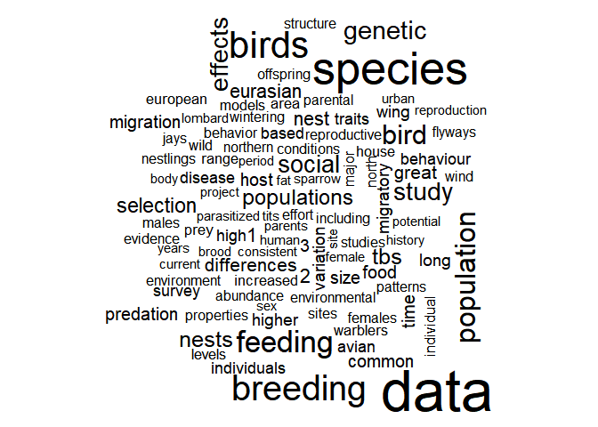
Data is the most common word which is quite logical for metadata of actual datasets. Let’s also have a look at a regular wordcloud.
with(data_words, wordcloud(word, n, max.words = 100))

As expected, the words seem more focused on ecology than when looking at scientific papers. DataONE is a gigantic data catalogue, where one could
-
study the results of such queries (e.g. meta studies of number of, say, versions by datasets)
-
or find data to integrate to a new study. If you want to download data from DataONE, refer to the download data vignette.
🔗 Conclusion
In this post, we used the rOpenSci fulltext package, and the DataONE
dataone package, to search for bird species names in scientific papers
and scientific open datasets. We were able to draw wordclouds
representing the diversity of topics of studies in which the birds had
been mentioned or studied. Such a search could be fun to do for your
favourite bird(s)! And in general, following the same approach you could
answer your own specific research question.
🔗 Scientific literature access
As a reminder, the pipeline to retrieve abstracts and titles of works mentioning a bird species was quite smooth:
species %>%
    tolower() %>%
    fulltext::ft_search() %>%
    fulltext::ft_get() %>%
    fulltext::ft_collect() %>%
    fulltext::ft_chunks(c("title", "abstract")) %>%
    fulltext::ft_tabularize() %>%
    dplyr::bind_rows()
fulltext gives you a lot of power! Other rOpenSci accessing literature
data include europepmc, R
Interface to Europe PMC RESTful Web Service;
jstor;
suppdata for extracting
supplemental information, and much
more.
🔗 Scientific data access… and publication with R
In this post we used the dataone
package to access data from
DataONE. That same package allows uploading data to DataONE. The
rOpenSci suite features the
rfigshare package for getting
data from, and publishing data to, Figshare.
For preparing your own data and its documentation for publication, check
out the EML package for writing
metadata respecting the Ecological Metadata Standard, and the unconf
dataspice project for
simpler metadata entry.
Explore more of our packages suite, including and beyond access to scientific literature &data and data publication, here.
🔗 No more birding? No, your turn!
This was the last post of this series, that hopefully provided an overview of how rOpenSci packages can help you learn more about birds, and can support your workflow. As a reminder, in this series we saw
-
How to identify spots for birding using open geographical data. Featuring
opencagefor geocoding,bboxfor bounding box creation,osmdatafor OpenStreetMap’s Overpass API querying,osmplotrfor map drawing using OpenStreetMap’s data. -
How to obtain bird occurrence data in R. Featuring
rebirdfor interaction with the eBird’s API, andaukfor munging of the whole eBird dataset. -
How to extract text from old natural history drawings. Featuring
magickfor image manipulation,tesseractfor Optical Character Recognition,cld2andcld3for language detection, andtaxize::gnr_resolvefor taxonomic name resolution. -
How to complement an occurrence dataset with taxonomy and trait information. Featuring
taxize, taxonomic toolbelt for R, andtraits, providing access to species traits data. -
How to query the scientific literature and scientific open data repositories. This is the post you’ve just read!
That’s a wrap! But now, don’t you hesitate to explore our packages suite for your own needs, and to share about your use cases of rOpenSci packages as a birder or not via our friendly discussion forum! Happy birding!

